The Achilles Heel of Vector Search: Filters
Table of Contents
- Overview
- Filtering Strategies in ANN Search
- How Vector Databases Support Filtering
- Filtered vs Unfiltered Search Performance
- Why Filtered Vector Search Is Slower than Traditional Filtering
- Filter Fusion: Encoding Filters into Embeddings
- References
Overview

Back in Q2 2024 at my previous role, I set out to answer what should have been a simple question for the whole company:
“Which vector database should I use?”
What started as a quick investigation turned into a deep dive—presenting my findings in talks and slides and questioning everything I thought I knew about indexes and search. Along the way, one discovery really blew me away: unlike a traditional RDBMS, adding a filter to a vector search often slows it down, not speeds it up.
In this post, we’ll unpack why filtered vector search is the Achilles’ heel of ANN:
- Pre-filtering: why “filter then search” often collapses back into brute force
- Post-filtering: how “search then filter” can miss results or blow up latency
- Integrated filtering: the cutting-edge tweaks (Qdrant’s filterable HNSW, Weaviate’s ACORN, Pinecone’s single-stage) that restore both speed and accuracy
We’ll also look at benchmark numbers from Faiss, Qdrant, Pinecone and Weaviate—and finish by exploring a promising new idea: filter fusion, where you encode metadata into your embeddings so that standard ANN search magically respects your filter without any extra step.
Note:
- X-axis:
mean_precision - Ratio 0.1: filter returns 10% of the original dataset (highly selective)
- Throughput chart: Y-axis is Throughput (QPS)
- Latency chart: Y-axis is P95 Latency (seconds)
Throughput Across Different Vector Databases

QPS Across Different Vector Databases

After running these benchmarks across six vector engines, two query modes (regular vs. 10%-filtered), and up to 16 search threads, a few clear patterns emerged:
- Thread scaling boosts throughput for all engines, but especially for Pinecone-p2 and Zilliz-AUTOINDEX. At 16 threads, Pinecone hits ~800 QPS unfiltered and ~600 QPS filtered Zilliz reaches ~750 QPS unfiltered and ~700 QPS filtered.
- Filtering often improves throughput on systems with integrated filtering:
- Pinecone-p2 and Zilliz-AUTOINDEX each see a ~1.2×–1.5× throughput bump under the 10% filter.
- Qdrant-HNSW shows a smaller gain thanks to its augmented-graph strategy.
- Brute-force or post-filter engines lose ground under a tight filter: LanceDB-IVF_PQ-ratio-0.1, OpenSearch-HNSW-ratio-0.1 and PGVector-HNSW-ratio-0.1 all dip in QPS when filtering, since they scan or oversample the subset.
- Tail latencies (P95) stay sub-100 ms in regular searches and often drop further with a 10% filter on integrated systems:
- Pinecone-p2 and Zilliz-AUTOINDEX shave 10–30 ms off P95, landing around 30–50 ms at 16 threads.
- Qdrant-HNSW-ratio-0.1 maintains similar latency, thanks to its adaptive planner.
- Brute-force fallbacks (LanceDB-IVF_PQ-ratio-0.1, OpenSearch-HNSW-ratio-0.1) can spike to 200–300 ms under filtering.
Bottom line: Engines with in-algorithm filtering not only preserve recall—they actually get faster, more predictable searches when filters prune the workload. Engines relying on pre- or post-filter fallbacks may see little benefit or even performance degradation when filters are applied.
Filtering Strategies in ANN Search
In vector search, a filter means we only want results from a subset of vectors (e.g. those whose category is “laptop”). Formally, vector filtering returns only vectors that meet a criterion and ignores all others. There are three broad strategies to combine filtering with ANN (Approximate Nearest Neighbor) search:
-
Pre-filtering (filter-then-search) First apply the metadata filter (e.g. via an inverted index), then run ANN on the resulting subset. Guarantees correctness, but if that subset is large you end up doing a near-linear scan (brute force).
-
Post-filtering (search-then-filter) First run ANN on the full dataset, then drop any results that fail the filter. Fast when filters are loose, but restrictive filters require oversampling (searching many more neighbors) to avoid missing matches, which hurts latency and recall.
-
In-algorithm filtering (integrated or single-stage) Modify the index or search logic so the ANN search itself only traverses or returns filtered vectors—e.g. Qdrant adds extra graph links, Weaviate’s ACORN does two-hop expansions, Pinecone merges metadata and vector indexes. This aims to combine pre-filter accuracy with ANN speed in a single pass.
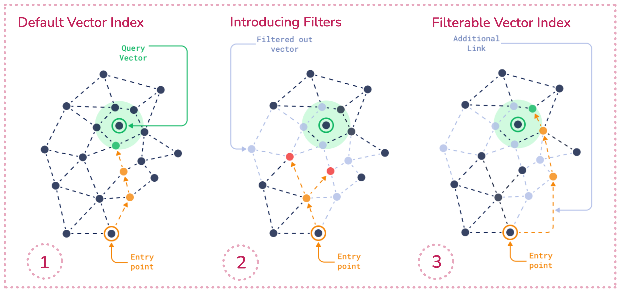
Filtering in HNSW (Graph-Based Indexes)
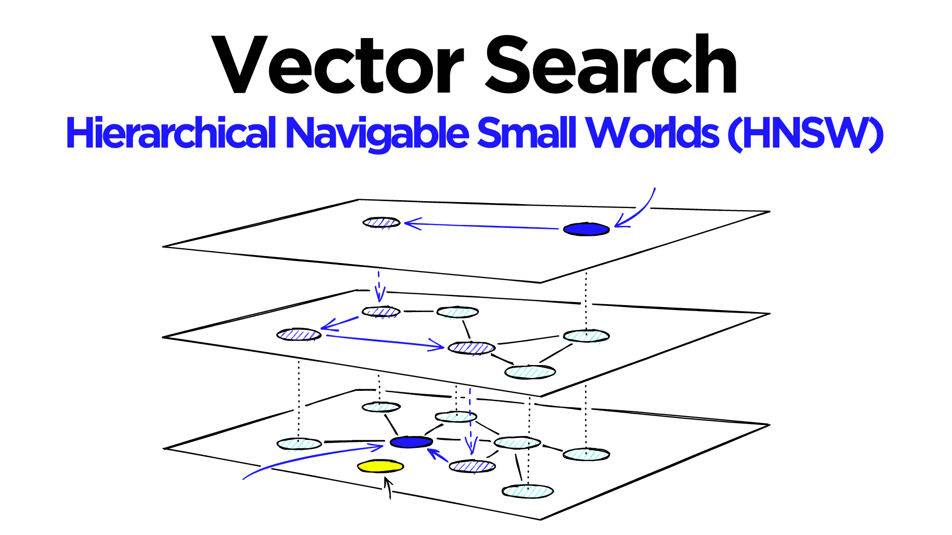
HNSW (Hierarchical Navigable Small World) is a popular graph index for ANN. Vectors are nodes connected by edges search traverses this graph greedily to find nearest neighbors. Applying filters here poses unique challenges:
Pre-Filtering
Skip the graph entirely when a filter is present: retrieve the IDs matching the filter (via a secondary metadata index) and do a linear scan or a small ANN build over that subset. Fast if the filtered subset is tiny, but performance degrades linearly as selection grows.
Post-Filtering
Run standard HNSW ignoring the filter, then discard non-matching neighbors. To ensure k valid results, you must oversample (e.g. request 10× k candidates if only 10 % match). This wastes distance computations and can miss results under tight filters.
Integrated Filtering
Make the HNSW graph itself filter-aware.
Approaches include:
- Sweeping (Weaviate): traverse normally but check each candidate’s filter, extending the search until enough valid points are found.
- Filterable HNSW (Qdrant): add extra intra-category links so filtered nodes don’t break graph connectivity.
- ACORN (Weaviate): maintain unpruned graph edges and use two-hop jumps to skip filtered-out nodes without disconnecting the graph.
HNSW Filtering Comparison
| Approach | Recall | Latency | Memory Overhead | Complexity |
|---|---|---|---|---|
| Pre-filtering | 100 % (subset) | O(subset size) | Low (metadata index) | Low |
| Post-filtering | Variable (<100 %) | O(ANN + oversample) | None | Low (tuning needed) |
| Integrated | ≈ 100 % | Near unfiltered (pruned) | High (extra links, edges) | High (algorithmic change) |
Filtering in IVF and IVF-PQ (Inverted Indexes)
 IVF (Inverted File) clusters data into coarse buckets IVF-PQ adds vector compression. Filtering here mirrors HNSW strategies but at the cluster level:
Pre-Filtering
Partition the IVF index by filter value (one index per category) or retrieve IDs via a metadata index and scan only those buckets. Efficient for tiny subsets impractical at scale or high-cardinality.
Post-Filtering
Perform standard IVF search (probe m nearest centroids), then drop non-matching items. Requires increasing nprobe under strict filters, which raises latency.
Integrated Filtering
Tag centroids with filter values and skip entire clusters that contain no valid vectors. This single-stage approach prunes the search space upfront, combining accuracy with speed.
IVF / IVF-PQ Filtering Comparison
| Approach | Recall | Latency | Memory/Index Overhead | Complexity |
|---|---|---|---|---|
| Pre-filtering | 100 % | O(subset size) | Metadata postings lists | Low |
| Post-filtering | Variable | O(IVF + oversample) | None | Low (parameter tuning) |
| Integrated | ≈ 100 % | Reduced by skipping irrelevant clusters | Cluster tag bitmasks | Medium to High |
How Vector Databases Support Filtering
- Faiss: Offers ID-mask support (bitsets) to skip candidates by metadata.
- Pinecone: Merges vector and metadata indexes into a single-stage filterable system.
- Qdrant: Uses a payload (inverted) index plus filterable HNSW, with a planner that picks brute-force or graph filtering based on selectivity.
- Weaviate: Combines HNSW + ACORN, falling back to flat scans on tiny subsets and two-hop graph jumps otherwise.
Filtered vs Unfiltered Search Performance
Faiss (IVF) – NeurIPS’23 Filtered Search Track: A Faiss baseline on 10 M vectors hit ~3 k QPS at 90 % recall. Optimized methods (e.g. multi-level IVF-PQ, graph hybrids) reached 30–40 k QPS at the same recall—a 10× gap.
Weaviate (HNSW) – Pre-ACORN vs ACORN: Pre-ACORN used flat scans for small filters and HNSW with inline sweeping for larger ones, leading to unpredictable latency under correlated filters. ACORN’s dense graphs and two-hop expansions stabilized performance and preserved recall on highly selective queries.
Pinecone – Single-Stage Filtering: On 1.2 M vectors (768-dim), unfiltered queries averaged 79 ms a 50 % selective filter dropped latency to 57 ms, and a 1 % filter to 51.6 ms (~35 % faster) by truly reducing search work.
Qdrant – Filterable HNSW: Qdrant’s planner picks graph filtering vs brute-force based on “filter cardinality.”
Why Filtered Vector Search Is Slower than Traditional Filtering
Given the performance challenges above, a fair question is: why is this so hard? Relational databases have provided fast filtering for decades using structures like B-trees, hash indexes, etc. If you ask SQL for SELECT * FROM products WHERE category = 'laptop' , it can use an index on the category column to fetch matching rows in almost constant time relative to the result size. So why can’t vector searches do top_k ANN ... WHERE category='laptop' just as easily?
The core issue is that vector search and metadata filtering are fundamentally different operations that are not trivially compatible. A few reasons:
- Index Mismatch: ANN indexes optimize for proximity, not boolean predicates—no native “category” tree.
- Graph Disconnects: Removing nodes fragments HNSW B-trees never face this.
- No Composite Key: You can’t jointly index (vector, metadata) as easily as relational DBs can on two columns.
- Approximation vs Exactness: ANN trades recall for speed filters demand exact matches, forcing extra work.
- Join-Like Complexity: Filtering + similarity is akin to a join between vector and metadata indexes, which is inherently more complex.
Filter Fusion: Encoding Filters into Embeddings
The FAISS team’s implementation in the Big-ANN Benchmark is particularly fascinating: by using unused bits of their 64-bit IDs to encode filter logic directly inside the IVF search loop, they achieved high-throughput filtered search without metadata callbacks or additional steps.
In their setup \((N = 10^7,\;d = 192)\), each vector also has sparse metadata in a CSR matrix called
\[M_{\mathrm{meta}}\;\in\;\mathbb{R}^{N\times v},\quad v \approx 2\times 10^5.\]Rather than testing membership with a callback, they:
- Allocate the low 24 ID bits for the vector index (since \(\log_{2}N \;=\;\log_{2}(10^{7})\;\approx\;23.25\;\longrightarrow\;24\text{ bits}\)
- Use the remaining 39 high bits to store a bitwise signature—each metadata term \(j\) gets a 39-bit random mask \(S_{j}\).
- For each vector \(i\) with metadata terms \(W_{i}\), compute its signature as \(\mathrm{sig}_{i}\;=\;\bigvee_{\,j\in W_{i}}S_{j}.\)
- For a query with terms \(w_{1},w_{2}\), compute its signature by
\(\mathrm{sig}_{q} \;=\;S_{w_{1}}\;\vee\;S_{w_{2}}.\) -
Inside IVF’s tight inner loop, discard any vector that doesn’t match all query terms:
\[\texttt{// skip if any query term is missing}\\ \quad\texttt{if }(\neg\mathrm{sig}_{i}\;\wedge\;\mathrm{sig}_{q})\neq0 \;\texttt{continue;}\]
Vectors lacking any query term are thrown out before any distance computation or metadata lookup—ruling out around 80 % of negatives in FAISS’s benchmarks. The clever bit: this “filter fusion” runs entirely inside the ANN engine, with no changes to the search algorithm itself.
Given the difficulties above, an intriguing solution is Filter Fusion – essentially, bake the filter criteria into the vector representation itself based on how the FAISS team did so. The idea is to avoid explicit filtering altogether by designing embeddings (or distance functions) such that an item that doesn’t meet the filter would never appear in the top results in the first place.
Imagine if for each vector, we could append a small descriptor of its metadata, and for each query, do the same. During similarity search, only vectors whose descriptors match the query’s descriptor closely would score highly. This way, the vector similarity metric itself enforces the filter. It’s like secretly encoding “category = laptop” within the vector coordinates.
Motivation & Intuition: If the vector space can incorporate both content and metadata, then a single nearest neighbor search can handle both aspects. This eliminates the need for separate filtering logic and ensures zero overhead for applying filters – the math of similarity takes care of it. It also potentially means we can use off-the-shelf ANN methods without modification, because we’re just searching in a slightly higher-dimensional space (original embedding + metadata encoding).
One simple approach to filter fusion is vector concatenation, let each document have:
- an embedding \(x_i \in \mathbb{R}^d\)
- a type label \(k_i \in \{1,\dots,T\}\)
Define the metadata one-hot vector \(m_i = e_{k_i} \;\in\; \{0,1\}^T\) and choose a metadata weight \(\alpha > 0\). Then augment each document and the query as
\[\tilde x_i = \begin{bmatrix} x_i \\[6pt] \alpha\,m_i \end{bmatrix} \;\in\;\mathbb{R}^{d+T}, \qquad \tilde q = \begin{bmatrix} q \\[6pt] \alpha\,e_c \end{bmatrix},\]Remark: In practice most ANN libraries use Cosine Similarity rather than Euclidean distance. If you \(\ell_2\)-normalize each augmented vector \(\tilde x_i\) and the query \(\tilde q\), then ranking by Cosine Similarity is equivalent to ranking by Euclidean distance, so the same filter-fusion trick applies directly.
\[\bigl\lVert \tilde x_i - \tilde q \bigr\rVert^2 = \underbrace{\lVert x_i - q\rVert^2}_{\text{content term}} \;+\;\alpha^2\, \underbrace{\lVert m_i - e_c\rVert^2}_{% \substack{0\;\text{if}\;k_i=c,\\2\;\text{otherwise}} }\,.\]Since
\[\lVert m_i - e_c\rVert^2 = \begin{cases} 0, & k_i = c,\\ 2, & k_i \neq c, \end{cases}\]any non-matching category incurs an extra penalty of \(2\alpha^2\). By choosing \(\alpha\) large enough, the top-\(k\) nearest neighbors will all satisfy \(k_i=c\), so one ANN query both retrieves and filters in one pass.
In simple terms lets say each data vector has a 256 dimension and we have a categorical filter with 10 possible values. We can allocate an extra 10 dimensions (a one-hot encoding for the category). A vector for an item in category 3 would have those extra 10 dims all 0 except a 1 in position 3. A query that requires category 3 would similarly have that one-hot in its vector. If we use standard Euclidean or cosine distance on the combined (266-dim) vectors, a candidate from a different category will have a large distance on the metadata dimensions, likely pushing it out of the top results. We can even exaggerate this by weighting the metadata dimensions more strongly (e.g. set the one-hot to some large value) so that any category mismatch dominates the distance. In effect, the nearest neighbor search “prefers” vectors of the same category because others are far away in those extra dimensions.
Filter Fusion in Practice (RAG Retrieval): Imagine a retrieval scenario with 1,000 mixed documents—manuals, FAQs, and tutorials—where only FAQs should be returned. By appending a high-weight one-hot slice that encodes each document’s type (and the query’s desired type) to the embedding, a single ANN search naturally ranks only FAQs at the top, removing the need for any separate filter step.
Maths Symbol to Code Variable
| Symbol | Code variable |
|---|---|
| \(x_i\) | doc_embeds[i] |
| \(m_i\) | type_onehot[i] / α |
| \(q\) | query_embed |
| \(e_c\) | np.eye(num_types)[desired_type] |
| \(\alpha\) | metadata_weight |
import numpy as np
from enum import IntEnum
from typing import Sequence


class DocType(IntEnum):
    MANUAL   = 0
    FAQ      = 1
    TUTORIAL = 2

    @classmethod
    def names(cls, types: Sequence[int]) -> list[str]:
        """
        Given a sequence of integer type codes, return the corresponding DocType names.
        """
        return [cls(t).name for t in types]

def filter_fusion_search(
    doc_embeds: np.ndarray,
    doc_types: np.ndarray,
    query_embed: np.ndarray,
    desired_type: DocType,
    metadata_weight: float = 10.0,
    top_k: int = 5
) -> tuple[np.ndarray, np.ndarray]:
    """
    Perform filter-fusion ANN search by appending weighted one-hot metadata.

    Args:
        doc_embeds: (N, d) array of document embeddings.
        doc_types: (N,) array of integer type labels (0...T-1).
        query_embed: (d,) query embedding.
        desired_type: integer label to filter for.
        metadata_weight: weight to amplify metadata dimensions.
        top_k: number of nearest neighbors to return.

    Returns:
        indices (top_k,) and distances (top_k,).
    """
    print("Filter fusion search")
    # One-hot encode document types
    num_types = int(doc_types.max()) + 1
    type_onehot = np.eye(num_types)[doc_types] * metadata_weight

    # Augment document embeddings
    aug_embeds = np.hstack([doc_embeds, type_onehot])

    # One-hot encode query type and augment query embedding
    query_meta = np.eye(num_types)[desired_type] * metadata_weight
    aug_query = np.hstack([query_embed, query_meta])

    # Compute L2 distances and get top_k results
    dists = np.linalg.norm(aug_embeds - aug_query, axis=1)
    idx = np.argsort(dists)[:top_k]

    print(f"Top-{top_k} indices: {idx}")
    print("Document types:", DocType.names(doc_types[idx]))
    print("Distances:", np.around(dists[idx], 3))

    assert np.all(doc_types[idx] == desired_type), \
        f"Filtering failed: some top-{top_k} docs are not type {desired_type}"
    print(f"Filtering success: all top-{top_k} docs match type {desired_type}.")

    return idx, dists[idx]

def post_filter_search(
    doc_embeds: np.ndarray,
    doc_types: np.ndarray,
    query_embed: np.ndarray,
    desired_type: DocType,
    top_k: int = 5
) -> tuple[np.ndarray, np.ndarray]:
    """
    Perform ANN search on embeddings, then filter the top results by desired_type.
    """
    print("Post-filter search")
    # 1. Nearest-neighbor on raw embeddings
    dists = np.linalg.norm(doc_embeds - query_embed, axis=1)
    idx = np.argsort(dists)

    # 2. Post-hoc filtering
    filtered = [i for i in idx if doc_types[i] == desired_type]
    top_filtered = np.array(filtered[:top_k])
    distances = dists[top_filtered]

    print(f"Post-filter top-{top_k} indices: {top_filtered}")
    print("Document types:", DocType.names(doc_types[top_filtered]))
    print("Distances:", np.around(distances, 3))

    # Ensure we have enough matches
    assert len(top_filtered) == top_k, \
        f"Filtering failed: only {len(top_filtered)} items of type {desired_type} found"
    print(f"Post-filtering success: all top-{top_k} docs match type {desired_type}.")
    return top_filtered, distances

def baseline_raw_search(
    doc_embeds: np.ndarray,
    doc_types: np.ndarray,
    query_embed: np.ndarray,
    top_k: int = 5
) -> tuple[np.ndarray, np.ndarray]:
    """
    Retrieve top_k nearest documents without any filtering.
    """
    print("Raw search without filter")
    # 1. Nearest-neighbor on raw embeddings
    dists = np.linalg.norm(doc_embeds - query_embed, axis=1)
    idx = np.argsort(dists)[:top_k]

    print(f"Raw top-{top_k} indices: {idx}")
    print("Document types:", DocType.names(doc_types[idx]))
    print("Distances:", np.around(dists[idx], 3))

    return idx, dists[idx]

if __name__ == "__main__":
    np.random.seed(42)
    N, d = 1000, 768
    # Correct document embeddings to match the number of documents
    doc_embeds = np.random.randn(N, d)
    # Randomly assign document types based on the DocType enum values
    doc_types = np.random.choice([t.value for t in DocType], size=N)
    query_embed = np.random.randn(d)

    # Test retrievals for FAQ (type=1)
    print("=== Raw Search ===")
    baseline_raw_search(doc_embeds, doc_types, query_embed)

    print("=== Post-Filter Search (FAQ) ===")
    post_filter_search(doc_embeds, doc_types, query_embed, desired_type=DocType.FAQ)

    print("=== Filter Fusion Search (FAQ) ===")
    filter_fusion_search(doc_embeds, doc_types, query_embed, desired_type=DocType.FAQ)
Output
=== Raw Search ===
Raw search without filter
Raw top-5 indices: [872 449 347 111 261]
Document types: ['TUTORIAL', 'MANUAL', 'MANUAL', 'MANUAL', 'MANUAL']
Distances: [35.385 35.761 35.939 35.965 36.072]
=== Post-Filter Search (FAQ) ===
Post-filter search
Post-filter top-5 indices: [835 494 881 681 912]
Document types: ['FAQ', 'FAQ', 'FAQ', 'FAQ', 'FAQ']
Distances: [36.127 36.222 36.416 36.42  36.47 ]
Post-filtering success: all top-5 docs match type 1.
=== Filter Fusion Search (FAQ) ===
Filter fusion search
Top-5 indices: [835 494 881 681 912]
Document types: ['FAQ', 'FAQ', 'FAQ', 'FAQ', 'FAQ']
Distances: [36.127 36.222 36.416 36.42  36.47 ]
Filtering success: all top-5 docs match type 1.`
Running the script on this toy RAG corpus clearly illustrates each approach:
- Raw Search (no filter) returns the closest documents regardless of type, mixing manual, FAQ, and tutorial entries.
- Post-Filter Search retrieves the top-5 nearest neighbors and then discards any non-FAQ documents, yielding only the desired category.
- Filter Fusion Search appends the category one-hot to embeddings so that a single ANN query directly surfaces only FAQ documents—matching the post-filter results without a separate step.
By concatenating metadata as weighted dimensions, off-the-shelf ANN can perform filtered search in one pass, eliminating extra filter logic which should give us gains in terms of latency/throughput which I will save for a separate blog post.
Limitations of Embedding-Level Filter Fusion
While embedding-level filter fusion streamlines retrieval, it has several practical drawbacks:
-
Dimensional explosion: Appending one-hot slices for each category or filter column increases embedding size linearly. High-cardinality fields (thousands of unique values) can bloat vectors and slow down ANN indexing and search.
-
Multi-column filters: Concatenating separate one-hot encodings for multiple attributes (e.g., category, region, user role) multiplies dimensionality and requires careful weight balancing across different metadata types.
-
Range and temporal queries: Encoding ordinal or continuous filters (dates, numeric ranges) as one-hot is infeasible. You’d need alternative schemes (e.g., positional encodings, bucketing, or learned embeddings) to approximate range semantics, which adds complexity.
-
Weight tuning challenges: Choosing the right metadata_weight is a trade‑off between strict filtering and semantic relevance. Too low a weight yields false positives; too high a weight can overshadow content similarity and hurt recall.
-
Dynamic metadata updates: If metadata changes frequently (e.g., document status, timestamps), embeddings must be regenerated or ID‑based signatures recalculated, complicating real-time systems.
-
Interpretability and maintenance: Mixing metadata with content dimensions makes embeddings harder to interpret and debug. Any change in metadata schema often requires re-indexing or modifying the fusion logic.
References
- Filtered Vector Search: The Importance and Behind the Scenes
- The Missing Where Clause in Vector Search
- FAISS Paper
- How we speed up filtered vector search with ACORN
- A Complete Guide to Filtering in Vector Search - Qdrant
- Big ANN: NeurIPS 2023
- Filtering Data in OpenSearch
- Efficient filtering in OpenSearch vector engine